How to Use the DGET Function in Excel

DGET is a straightforward lookup function designed to retrieve a single value from a column in a table or database. It’s particularly useful for extracting a single point of data from a large spreadsheet, saving you from scrolling endlessly to find the info you need.

In this guide, I’ll walk you through the function’s syntax, show you some real-world examples, and discuss some of its pros and cons.

The DGET Syntax

Here’s the syntax for this function:

=DGET(a,b,c)

where

• a is the database—the range of cells (including the column headings) from which the formula will retrieve the data. The database must be presented in such a way that the categories (such as name, address, and age) are in columns, and the data (the records) are in rows.
• b is the field—the column category label that Excel will use to search for the output. This can be a word or string of words in double quotes (DGET is not case-sensitive), or a cell reference.
• c are the criteria—the range of cells containing the conditions for the lookup.

All three arguments for this function are required, meaning if you omit any, Excel will return a #VALUE! error.

So that I can explain this to you more clearly, here are some examples.

Example 1: One Criterion

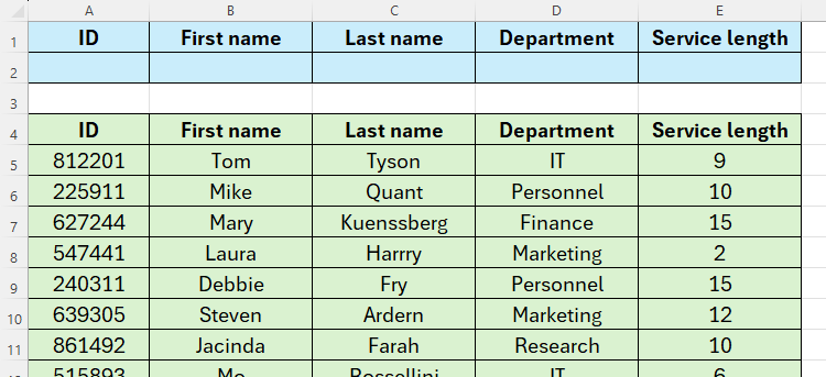
Let’s start with this very basic example, which is a list of employees’ IDs, names, departments, and lengths of service.

The Spreadsheet Setup

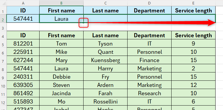
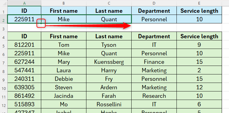
The blue table at the top is my retrieval table, and the green table underneath is my database. The aim is to return an employee’s first name, last name, department, and service length in the blue retrieval table when I input their ID into cell A2.

Before I show you how to pull data from the green database table to the blue retrieval table, let me highlight a few important things in the screenshot above:

• In my green database table, each column is a different category, and each row is a different record.
• Both the database and the retrieval tables contain the same headings.
• Because each employee has a unique ID, I know the DGET function won’t return the #NUM! error.

Adding a Drop-Down List

To save me from having to type an employee’s ID into cell A2 each time, I will create a drop-down list of these numbers.

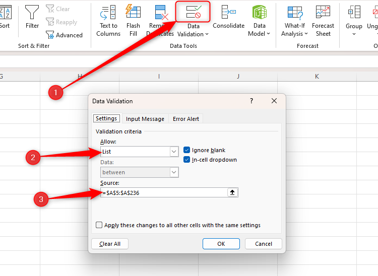
If you want to do the same, select the relevant cell, and click “Data Validation” in the Data tab. Then, choose “List” in the Allow field, and select the cells containing the drop-down data in the Source field. In my example, even though I only have 175 IDs in my database, I have extended the data validation list to cell A236, so that any further IDs I add will be included in my drop-down.

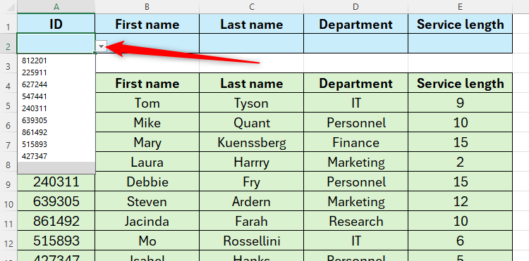
Notice how cell A2 now contains a drop-down arrow, which can be clicked to show the full list of IDs.

With one of these IDs selected, I’m now ready to begin my DGET retrieval.

The DGET Formula

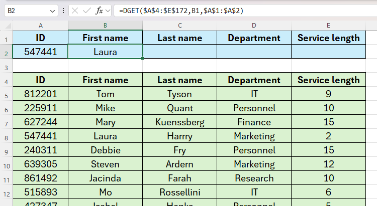
In cell B2, I will type:

=DGET($A$4:$E$172,B1,$A$1:$A$2)

because cells A4 to E172 represent my database, the value in B1 (first name) is the category or field I want Excel to search for, and cells A1 and A2 (the category name “ID” and the ID in cell A2 selected from my drop-down) are the criteria. When I press Enter, I can see that Excel has successfully retrieved the first name based on the ID in cell A2.

Arguments a and c contain dollar ($) symbols before the column and row references because they are absolute references. In other words, these references will never change—I will always use the ID to create the lookup, and the database will always be in these cells. I added these dollar symbols by pressing F4 after adding each reference to my formula.

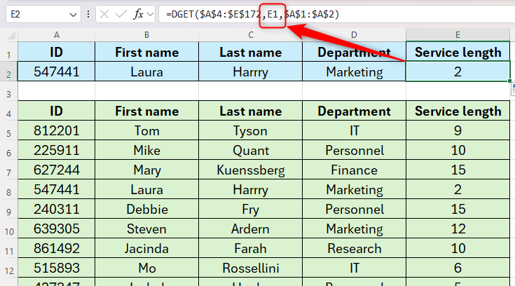
However, I deliberately left argument b as a relative reference, since I will now use Excel’s fill handle to apply the same formula to the remaining categories in my retrieval table (last name, department, and service length).

Notice how the formula in cell E2 retrieves the field name from cell E1 as a result, while the database and criteria references have remained fixed.

I can now choose a different ID in cell A2 using the drop-down I created to retrieve the details of other employees.

Example 2: Multiple Criteria

To make the lookup more specific—useful if your DGET keeps returning the #NUM! error due to there being more than one match—you can use more than one criterion in argument c.

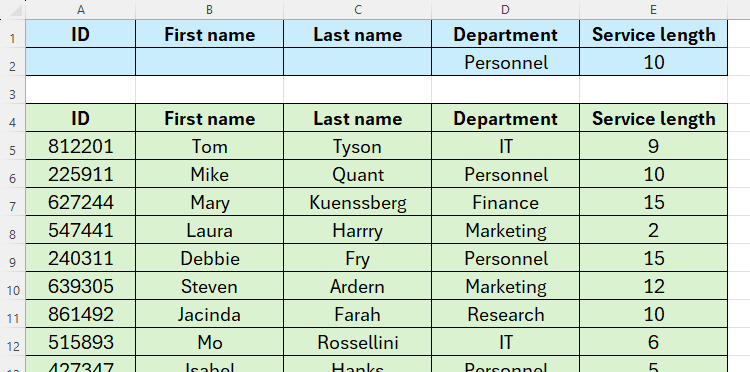
Here, I want to return the ID, first name, and last name of an employee who I know has worked in the Personnel department for ten years but whose name I can’t quite remember.

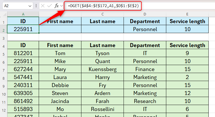
First, in cell A2, I will type:

=DGET($A$4:$E$172,A1,$D$1:$E$2)

where cells A4 to A172 contain my database, cell A1 is the category, and cells D1 to E2 contain my two criteria. In effect, Excel is creating an AND logical sequence between cells D2 and E2 to define my criteria.

Because I fixed my database and criteria references, but left the category reference relative, I can duplicate the formula in the remaining cells of my retrieval table to remind myself of this employee’s name.

If you’re more familiar with VLOOKUP, you might have noticed that you can use DGET to retrieve data from the right or left of where you are entering your formula, a flexibility that VLOOKUP does not offer.

You can also create an OR logical sequence by adding another row to your retrieval table. For example, if I knew that someone had been employed for one or two years, but I couldn’t remember their name, I would type
1
in cell E2,
2
in cell E3, and extend argument
c
to cover cells E1 to E3. Excel would then look for and return an entry that had either 1
or
2 as the service length. However, if more than one person fulfilled these criteria, Excel would return the #NUM! error.

The Pros of Using DGET

You may be wondering, “Why should I use DGET when there are other, more advanced functions?” Well, here are some benefits of using this tool:

• DGET has only three arguments, making it much more straightforward to use than other Excel lookup functions.
• The DGET function is an old-school tool! This means that, unlike some of its more modern counterparts (like XLOOKUP), it’s compatible with older versions of Excel.
• Where VLOOKUP can only perform a right-looking search, DGET can return values to the left of the lookup column.
• DGET adapts instantly to criteria changes.
• This function works with both text and numbers.

The Cons of Using DGET

On the other hand, while DGET’s simplicity makes it easy to use, it also means that there are some drawbacks to be aware of:

---

In this article, I’ve discussed DGET, VLOOKUP, HLOOKUP, and XLOOKUP, some of Excel’s best-known lookup functions. However, it would be remiss of me not to mention INDEX and MATCH, which—when combined—are powerful, flexible, and adaptable alternatives.