Who knew that Microsoft Excel could act as a translator? Through Microsoft Translate Services, Excel can translate from one language to another (the TRANSLATE function) and detect another language already in a workbook (the DETECTLANGUAGE function).
You will only see these language functions (added in December 2024) if you’re using the Excel Windows or Mac desktop app as a Microsoft 365 subscriber, Excel for the web, or the Excel mobile app.
What Are the Syntaxes?
Before I show you some examples of each function in action, here are their syntaxes.
TRANSLATE
The TRANSLATE function has three arguments:
=TRANSLATE(a,b,c)
where
- a (required) is either the text to translate (embedded in double quotes), or a reference to the cell containing the text to translate.
- b (optional) is the source language code in double quotes (see the Language Codes section below). If you omit this argument, Excel will try to detect the language automatically. Although this is an optional argument, it’s best to include it (if you know the language and its code) to ensure an accurate translation.
- c (optional) is the target language in double quotes. If you skip this argument, Excel will use your system language as the target language. However, again, try to add a target language code for better translation outcomes.
If you don’t place the language code within double quotes, Excel will return the #NAME? error.
DETECTLANGUAGE
This function is much more straightforward, requiring only one argument:
=DETECTLANGUAGE(x)
where
- x is either the text to detect, embedded within double quotes, or a reference to the cell containing the text to detect.
Language Codes
Here are some of the language codes from Microsoft’s longer list of codes. Remember that all language codes in your formula must be in double quotes.
|
Code |
Language |
|---|---|
|
“en” |
English |
|
“es” |
Spanish |
|
“fr” |
French |
|
“de” |
German |
|
“zh-chs” |
Mandarin (simplified) |
|
“ru” |
Russian |
|
“ar” |
Arabic |
Examples of TRANSLATE in Action
Let me show you the TRANSLATE function using two real-world examples. The first is a basic translation of several cells in Excel, while the second example shows you how to use the TRANSLATE function dynamically with a drop-down list.
Example 1: Translating Text in Cells
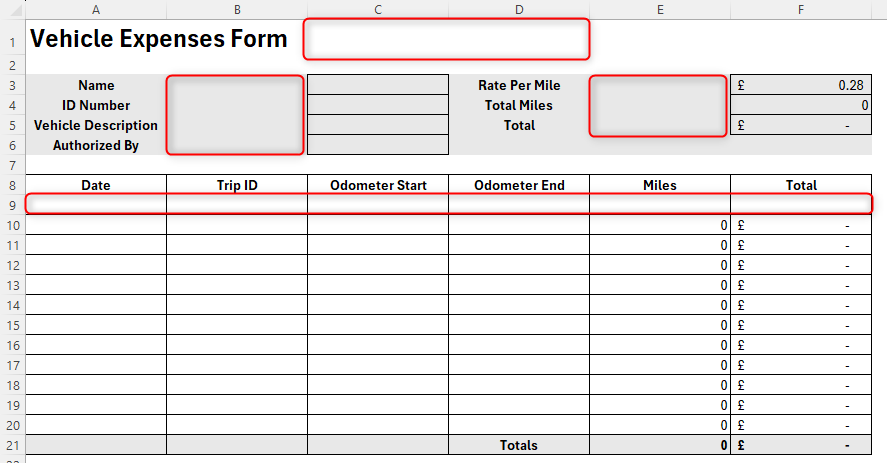
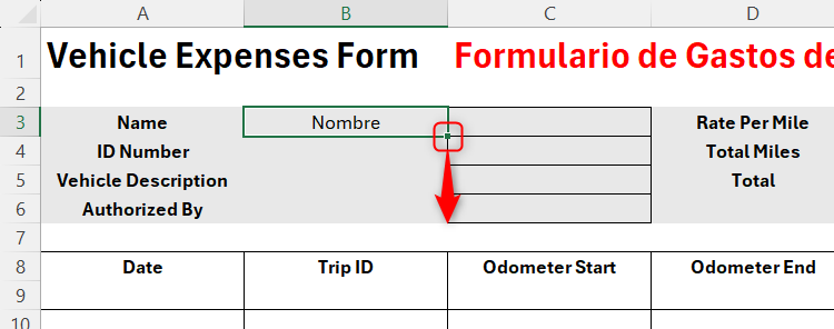
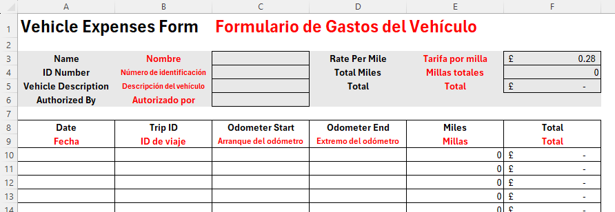
Let’s say you have a vehicle expenses form, and you want to translate the form’s title, totals section, and table headers from English into Spanish.
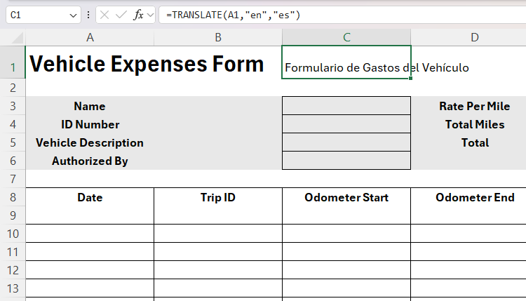
Starting in cell C2, type:
=TRANSLATE(A1,"en","es")
and press Enter.
Now, use the format painter tool to apply the formatting of the English title to the Spanish title. You can also apply a red font to distinguish between the two languages.
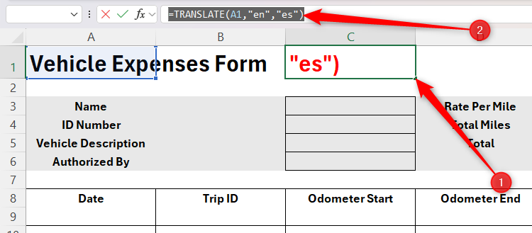
You’re now ready to translate the next section of the form. First, select cell C1, and select and copy (Ctrl+C) the formula in the formula bar.
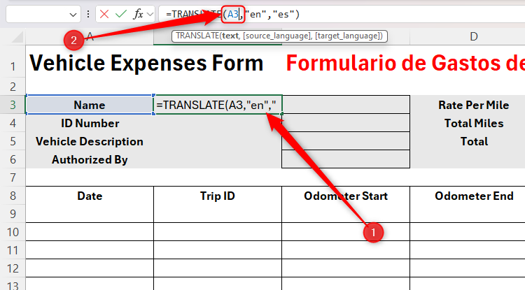
Now, select cell B3, paste (Ctrl+V) the copied formula into the formula bar, and change the first argument to reference cell A3, before pressing Enter.
Now, use the fill handle to apply the same relative formula to cells B4 to B6.
To finish this section, copy and paste the formula into cell E3, and use the fill handle again.
Because some of the Spanish translations contain more characters than their English counterparts, adjust the font sizes (or, if you prefer, the column widths) so that they fit nicely into their respective cells. Remember to also change the font colors to red for consistency.
Finally, follow the same process to translate your table headers.
Example 2: Selecting a Translating Language From a Drop-Down List
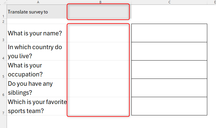
This survey contains some questions that the respondent needs to fill in. Your aim is to create a drop-down list of languages so that the respondent can choose the language in which they want to see the questions.
The first step is to create the list of available languages. Let’s say you want to offer Spanish, French, and Arabic as the options. Open Sheet 2 using the tabs at the bottom of your Excel window. Then, type each of those languages into separate rows in column A and their corresponding codes in column B.
Because you’re going to refer to the cells containing these language codes, rather than type them directly into your formula, you don’t need to embed them within double quotes.
Now, in cell C1, type:
=TRANSLATE(A1,"en",B1)
Press Enter, and then use the fill handle to populate the remaining rows.
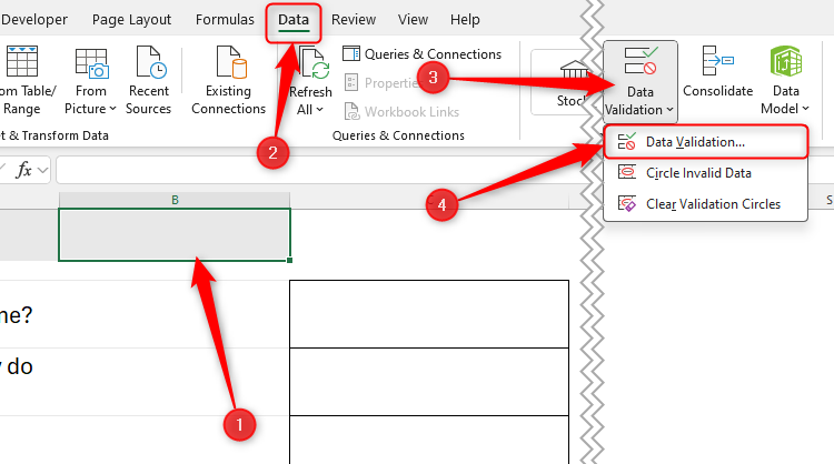
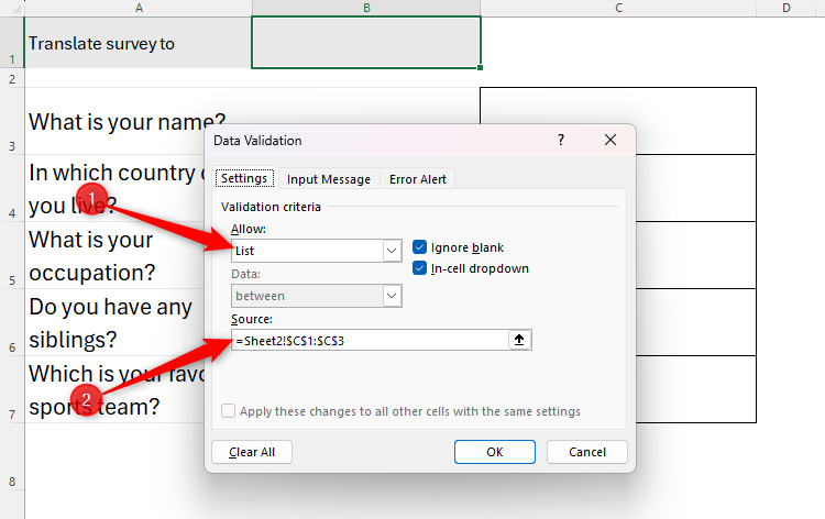
It’s now time to create the drop-down list in Sheet 1. Select the cell where the drop-down will go, click the “Data Validation” drop-down icon in the Data tab, and select “Data Validation.”
Select “List” in the Allow field, and after placing your cursor in the Source field, select the three cells containing the translations of the chosen languages (cells C1 to C3 in Sheet 2).
When you click “OK,” you’ll see a drop-down list appear at the top of your survey, which, when clicked, displays the words Spanish, French, and Arabic in their respective languages.
To prepare your spreadsheet for the final step, select one of the languages from this list.
You’re now ready to translate your questions into the selected language. In cell B3, type (or copy and paste) the following formula:
=TRANSLATE(A3,"en",XLOOKUP($B$1,Sheet2!$C$1:$C$3,Sheet2!$B$1:$B$3))
where
- A3 is the cell containing the text you want to translate (the survey question),
- “en” is the source language of that text, and
- the third argument is an XLOOKUP formula that takes the selected language, looks for that in your table in Sheet 2, and returns the language code.
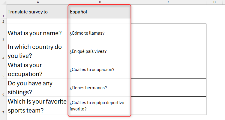
When you press Enter, the first question translates into the language you selected from the drop-down list earlier. Then, use the fill handle to apply the formula to the remaining questions in your survey.
Reduce the font size slightly in cells B3 to B7 to account for the fact that some translations may contain more characters than the questions in English.
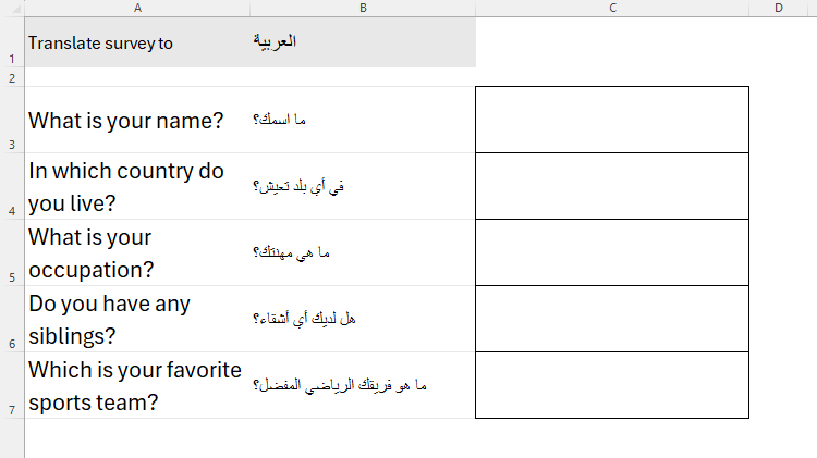
Finally, change the language in your drop-down menu to see the translations magically change accordingly!
An Example of DETECTLANGUAGE in Action
If your spreadsheet contains data in many languages, you might find it useful to use Excel’s DETECTLANGUAGE function.
Suppose you have received this spreadsheet containing three non-English sentences in cells A1 to A3, and you want Excel to identify their languages.
In cell B1, type:
=DETECTLANGUAGE(A1)
and press Enter. Then, use the fill handle to copy this formula to cells B2 and B3.
Column B now contains the language codes for each of these sentences. If you’re unsure what these codes represent, you can see the full list on Microsoft’s translator language support page.
As well as translating in Excel, you can also translate text in a Microsoft Word document. To translate a section of a file, select the relevant text, and click Review > Translate > Translate Selection. This opens the Translator pane, where you can choose a target language. Alternatively, to open a translated copy of a whole document, click Review > Translate > Translate Document.
