Apple Numbers isn’t as popular as Excel, but it’s a powerful spreadsheet application that offers all the essential features you’d expect. If you’re thinking about making the switch, here are some functions and features you should master.
1 Add a Dropdown List to a Cell
A dropdown list helps ensure consistent data entry in a spreadsheet column and reduces the chances of errors by others working on it. It allows you to select from predefined options, such as “completed” or “in progress,” for columns tracking project statuses. By limiting choices, dropdown lists also make the spreadsheet easier to manage.
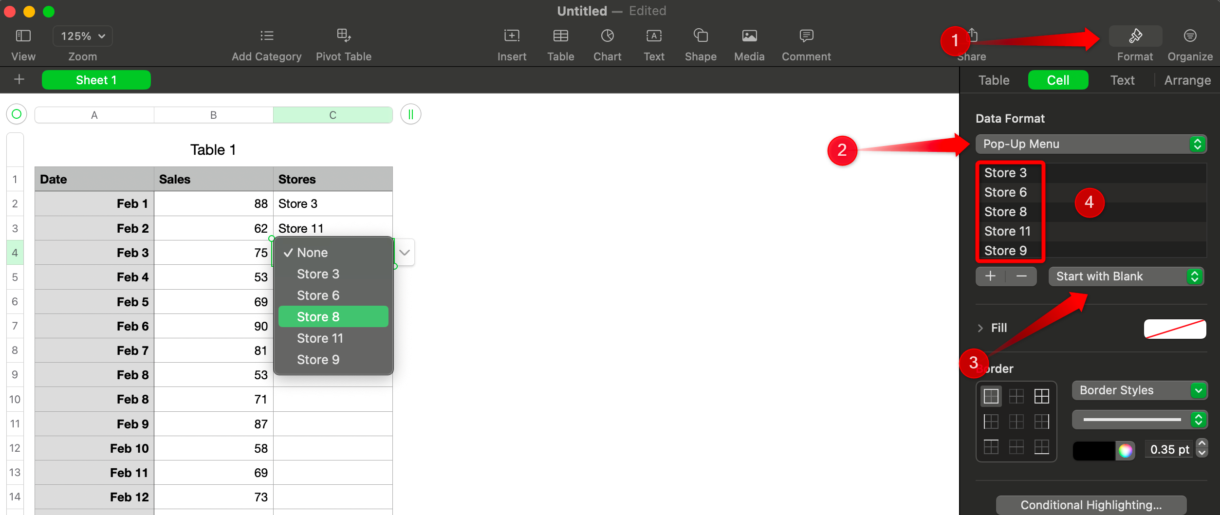
To create a dropdown list, select the cell or range of cells where you want a value to appear. Then, click the “Format” button in the top-right corner and go to the “Cell” tab. Set the data format to “Pop-Up Menu,” and enter the desired options to populate the dropdown. You can also reorder the options to suit your needs.
2 Predict Based on Existing Data
Apple Numbers allows you to make data-driven predictions in your spreadsheet using the Trendlines and Forecasting feature. When your data is well-organized and shows a clear relationship between variables, like months versus sales, you can easily spot trends, forecast sales, plan budgets, and more.
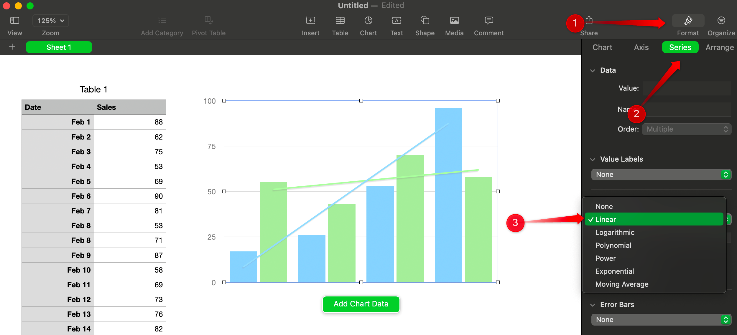
To use this feature, select the data you want to analyze and create a chart, such as a line or scatter plot. Next, click on the chart, open the “Format” panel, select “Series,” and select “Linear.” Numbers lets you predict data using linear, polynomial, exponential, and other models. You can easily extend the trendline to estimate future values.
3 Color-Code Cells Using Conditional Logic
Like Excel, Numbers allows you to format cells based on specific criteria using color coding. This helps you visually highlight important data points, making it easier to spot trends, outliers, or key details at a glance. Whether you need to flag values exceeding a limit, data within a specific range, or overdue tasks, color-coding makes it simple.
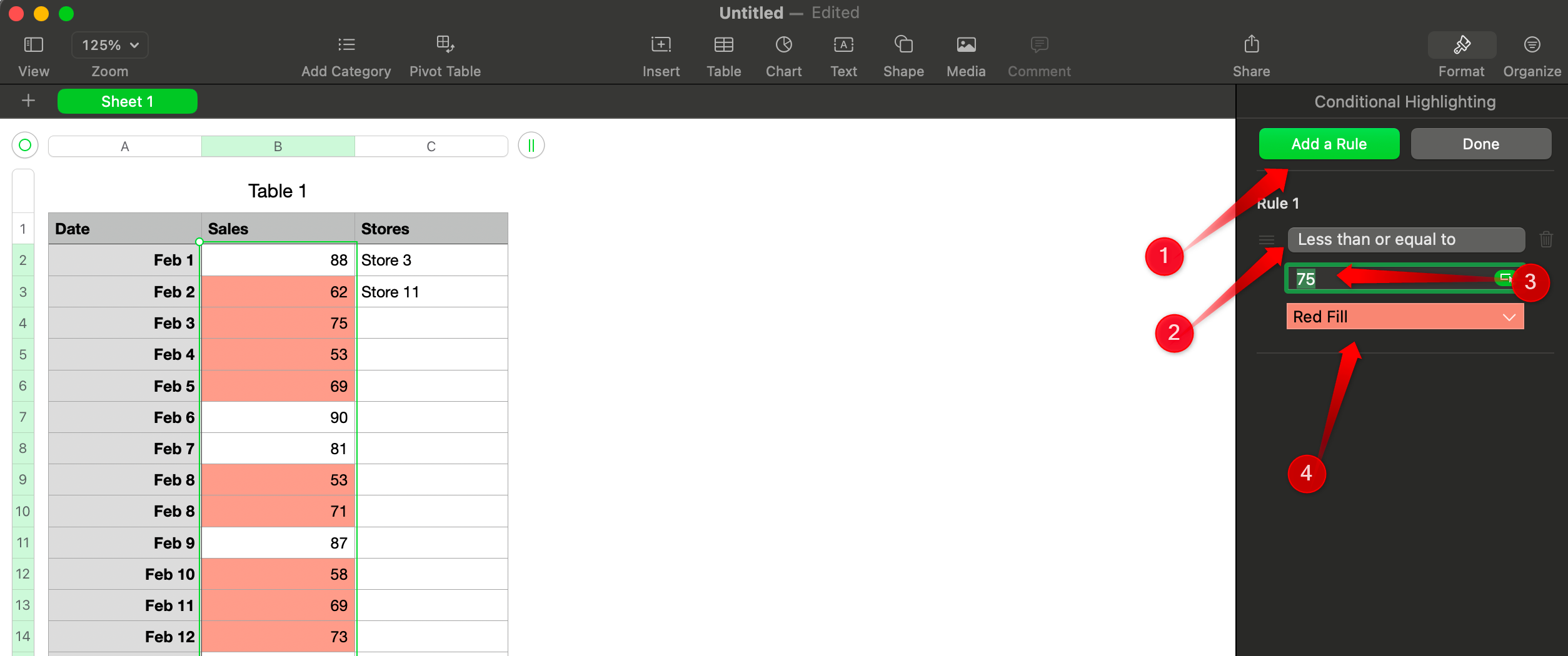
To apply color-coding, select the cells or range you want to format, click the “Format” button in the toolbar, and go to the “Cell” tab. Under Conditional Highlighting, click “Add a Rule,” then choose the condition you want to apply and set the value. After that, pick a fill color, text color, or both to highlight the cells that meet the criteria.
If you want to apply multiple conditions to different ranges or criteria, you can use different color coding within the same range.
4 Freeze Header Rows or Columns
In a spreadsheet, headers or labels provide context for the data in columns or rows. However, as a dataset grows, headers and rows can become hidden when you scroll down or to the right, making it difficult to identify which column corresponds to what data. To solve this issue, Numbers lets you freeze headers, rows, and columns so they stay visible as you scroll.
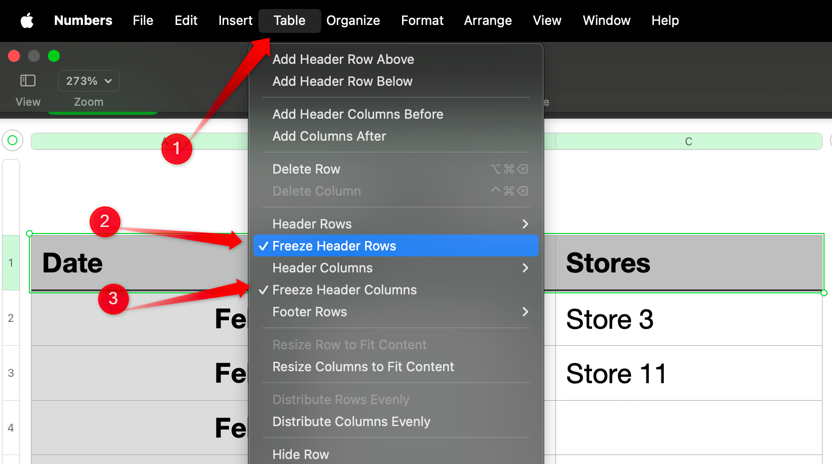
Select the row(s) or column(s) you want to freeze, typically the top row or leftmost column with the headers. Then, go to the “Table” menu in the toolbar and choose either “Freeze Header Rows” or “Freeze Header Columns,” depending on your needs. With this setting, the frozen rows and columns will stay in place as you scroll through your spreadsheet.
To unfreeze the rows or columns, return to the “Table” menu and uncheck the “Freeze Header Rows” or “Freeze Header Columns” option.
5 Count Checked and Unchecked Boxes
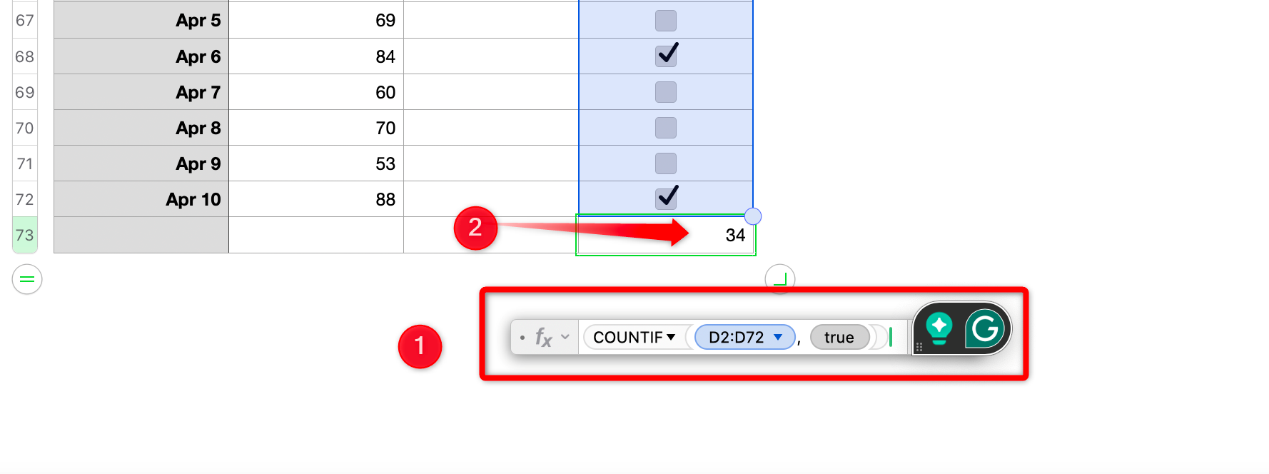
When using Numbers to track attendance, monitor task statuses, or manage stock levels, you can use checkboxes to mark or unmark items. However, with large datasets, manually counting checked and unchecked boxes can be difficult. Fortunately, you can automate this process using the COUNTIF function, which works the same way in Microsoft Excel.
The syntax for the COUNTIF function is as follows:
=COUNTIF(Range, TRUE/FALSE) Here, “Range” refers to the cells containing checkboxes. To count the number of checked boxes, use TRUE. To count unchecked boxes, use FALSE.
6 Merge Data of Two Columns
We often work with datasets that have data spread across multiple columns, but we need to combine it into a single column. This could include combining first, middle, and last names or merging parts of an address, such as house numbers, streets, and cities. Instead of integrating this data manually, you can easily automate the process.
To merge data from two columns, go to the first cell where you want the combined data and enter this formula:
=A1 & " " & B1 Here, A1 and B1 refer to the first cells in the two columns you want to combine, and the & operator joins their values. The ” ” adds a space between them.
You can then drag the fill handle down the column to apply the formula to all rows. Alternatively, you can use the CONCATENATE function, which performs the same task. If you’re new to working with spreadsheets, Apple Numbers might be a better option. It’s one area where Apple Numbers stands out compared to Excel.
7 Remove Blank Rows to Declutter a Worksheet
Blank rows can make your worksheet more difficult to read and analyze. To keep your spreadsheet easier to navigate, you must remove them. However, manually removing them can be time-consuming, especially if the dataset is large. Although Apple Numbers doesn’t have a built-in feature for this, you can use several workarounds to accomplish the task.
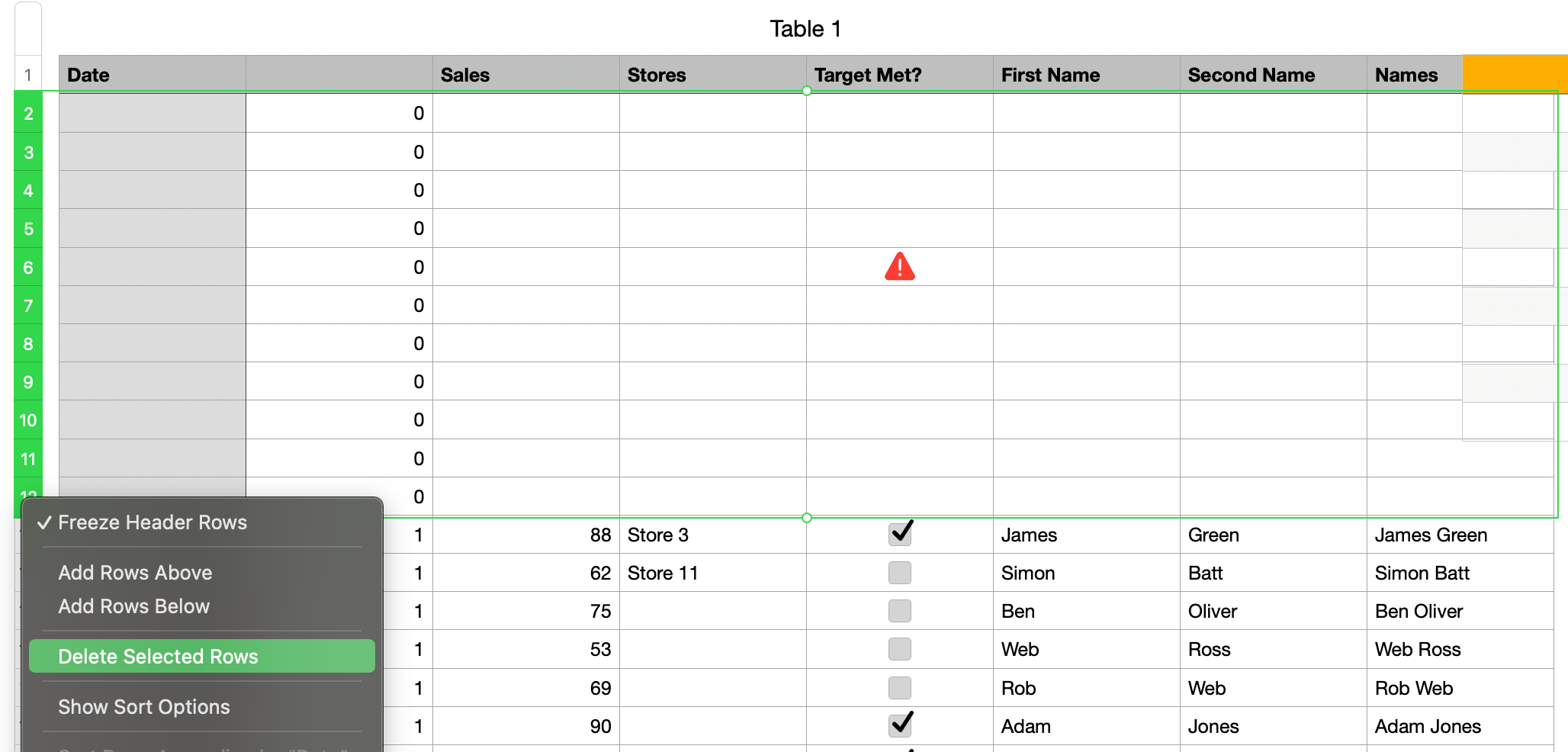
Here’s one of the simplest ways to remove blank rows. Add a new helper column to your table and enter the formula IF(ISBLANK(column), 0, 1) in the first cell, where “column” refers to the column containing empty rows. This will place “0” in empty cells and “1” in non-empty ones of the helper column.
To remove the blank rows, right-click the new column, select “Sort Ascending,” choose all the rows with “0”, and click “Delete Selected Rows.”
8 Lock Tables to Prevent Accidental Changes
When collaborating on a spreadsheet, you might want to protect certain cells from editing to avoid accidental changes. While you can lock individual cells in Excel, Apple Numbers only allows you to lock entire tables or spreadsheets. This ensures that important data, formulas, or formatting in specific tables remain secure while others can still edit the rest of the sheet.
To lock a table in Apple Numbers, select the table you wish to protect, go to the “Arrange” tab in the top menu, and select “Lock.” This will lock all cells within that table, leaving other tables editable. If you later want to unlock the table, return to the “Arrange” tab again and click “Unlock” from the menu.
These are a few basic tips and tricks you should know if you’re new to using Apple Numbers. While these cover the basics, they’re just the starting point. To maximize the potential of Apple Numbers, dedicate time to exploring its advanced features and formulas. It has all the tools to become your primary spreadsheet app on macOS.

